A meme floating around these days takes a swing at the existence of the electoral college stating "land doesn't vote, people do". While I don't subscribe to either side of that particular argument, the meme does a great job of highlighting how population data is essential for any analysis involving people. As such it is important to have a reliable source for population data.
Luckily in the U.S. we have the census bureau. Census.gov provides several datasets for our consumption. You can retrieve census data automatically using a pandas dataframe.
census.gov data
import pandas as pd

df = pd.read_excel('https://www2.census.gov/programs-surveys/popest/tables/2010-2019/state/totals/nst-est2019-01.xlsx')

df.head(10)
|
table with row headers in column A and column headers in rows 3 through 4. (leading dots indicate sub-parts) |
Unnamed: 1 |
Unnamed: 2 |
Unnamed: 3 |
Unnamed: 4 |
Unnamed: 5 |
Unnamed: 6 |
Unnamed: 7 |
Unnamed: 8 |
Unnamed: 9 |
Unnamed: 10 |
Unnamed: 11 |
Unnamed: 12 |
| 0 |
Table 1. Annual Estimates of the Resident Popu... |
NaN |
NaN |
NaN |
NaN |
NaN |
NaN |
NaN |
NaN |
NaN |
NaN |
NaN |
NaN |
| 1 |
Geographic Area |
2010-04-01 00:00:00 |
NaN |
Population Estimate (as of July 1) |
NaN |
NaN |
NaN |
NaN |
NaN |
NaN |
NaN |
NaN |
NaN |
| 2 |
NaN |
Census |
Estimates Base |
2010 |
2011.0 |
2012.0 |
2013.0 |
2014.0 |
2015.0 |
2016.0 |
2017.0 |
2018.0 |
2019.0 |
| 3 |
United States |
308745538 |
308758105 |
309321666 |
311556874.0 |
313830990.0 |
315993715.0 |
318301008.0 |
320635163.0 |
322941311.0 |
324985539.0 |
326687501.0 |
328239523.0 |
| 4 |
Northeast |
55317240 |
55318443 |
55380134 |
55604223.0 |
55775216.0 |
55901806.0 |
56006011.0 |
56034684.0 |
56042330.0 |
56059240.0 |
56046620.0 |
55982803.0 |
| 5 |
Midwest |
66927001 |
66929725 |
66974416 |
67157800.0 |
67336743.0 |
67560379.0 |
67745167.0 |
67860583.0 |
67987540.0 |
68126781.0 |
68236628.0 |
68329004.0 |
| 6 |
South |
114555744 |
114563030 |
114866680 |
116006522.0 |
117241208.0 |
118364400.0 |
119624037.0 |
120997341.0 |
122351760.0 |
123542189.0 |
124569433.0 |
125580448.0 |
| 7 |
West |
71945553 |
71946907 |
72100436 |
72788329.0 |
73477823.0 |
74167130.0 |
74925793.0 |
75742555.0 |
76559681.0 |
77257329.0 |
77834820.0 |
78347268.0 |
| 8 |
.Alabama |
4779736 |
4780125 |
4785437 |
4799069.0 |
4815588.0 |
4830081.0 |
4841799.0 |
4852347.0 |
4863525.0 |
4874486.0 |
4887681.0 |
4903185.0 |
| 9 |
.Alaska |
710231 |
710249 |
713910 |
722128.0 |
730443.0 |
737068.0 |
736283.0 |
737498.0 |
741456.0 |
739700.0 |
735139.0 |
731545.0 |
Next we need to clean up our data
new_header = df.iloc[2]
new_header
table with row headers in column A and column headers in rows 3 through 4. (leading dots indicate sub-parts)               NaN
Unnamed: 1                                                                                                              Census
Unnamed: 2                                                                                                      Estimates Base
Unnamed: 3                                                                                                                2010
Unnamed: 4                                                                                                                2011
Unnamed: 5                                                                                                                2012
Unnamed: 6                                                                                                                2013
Unnamed: 7                                                                                                                2014
Unnamed: 8                                                                                                                2015
Unnamed: 9                                                                                                                2016
Unnamed: 10                                                                                                               2017
Unnamed: 11                                                                                                               2018
Unnamed: 12                                                                                                               2019
Name: 2, dtype: object
Next we only want state an territory data so we can remove any aggregate rows or non-data rows from our dataset
Looking at the above dataframe we can see that our states and territories start at row 10. We can therefore discard everything above row 10
df = df[10:]

df.head()
|
table with row headers in column A and column headers in rows 3 through 4. (leading dots indicate sub-parts) |
Unnamed: 1 |
Unnamed: 2 |
Unnamed: 3 |
Unnamed: 4 |
Unnamed: 5 |
Unnamed: 6 |
Unnamed: 7 |
Unnamed: 8 |
Unnamed: 9 |
Unnamed: 10 |
Unnamed: 11 |
Unnamed: 12 |
| 10 |
.Arizona |
6392017 |
6392288 |
6407172 |
6472643.0 |
6554978.0 |
6632764.0 |
6730413.0 |
6829676.0 |
6941072.0 |
7044008.0 |
7158024.0 |
7278717.0 |
| 11 |
.Arkansas |
2915918 |
2916031 |
2921964 |
2940667.0 |
2952164.0 |
2959400.0 |
2967392.0 |
2978048.0 |
2989918.0 |
3001345.0 |
3009733.0 |
3017804.0 |
| 12 |
.California |
37253956 |
37254519 |
37319502 |
37638369.0 |
37948800.0 |
38260787.0 |
38596972.0 |
38918045.0 |
39167117.0 |
39358497.0 |
39461588.0 |
39512223.0 |
| 13 |
.Colorado |
5029196 |
5029319 |
5047349 |
5121108.0 |
5192647.0 |
5269035.0 |
5350101.0 |
5450623.0 |
5539215.0 |
5611885.0 |
5691287.0 |
5758736.0 |
| 14 |
.Connecticut |
3574097 |
3574147 |
3579114 |
3588283.0 |
3594547.0 |
3594841.0 |
3594524.0 |
3587122.0 |
3578141.0 |
3573297.0 |
3571520.0 |
3565287.0 |
We can also see when reviewing the dataset that there are 5 non-data rows at the end of the dataset. We can discard these rows as well
df = df[:-5]

df.tail(10)
|
table with row headers in column A and column headers in rows 3 through 4. (leading dots indicate sub-parts) |
Unnamed: 1 |
Unnamed: 2 |
Unnamed: 3 |
Unnamed: 4 |
Unnamed: 5 |
Unnamed: 6 |
Unnamed: 7 |
Unnamed: 8 |
Unnamed: 9 |
Unnamed: 10 |
Unnamed: 11 |
Unnamed: 12 |
| 51 |
.Texas |
25145561 |
25146091 |
25241971 |
25645629.0 |
26084481.0 |
26480266.0 |
26964333.0 |
27470056.0 |
27914410.0 |
28295273.0 |
28628666.0 |
28995881.0 |
| 52 |
.Utah |
2763885 |
2763891 |
2775332 |
2814384.0 |
2853375.0 |
2897640.0 |
2936879.0 |
2981835.0 |
3041868.0 |
3101042.0 |
3153550.0 |
3205958.0 |
| 53 |
.Vermont |
625741 |
625737 |
625879 |
627049.0 |
626090.0 |
626210.0 |
625214.0 |
625216.0 |
623657.0 |
624344.0 |
624358.0 |
623989.0 |
| 54 |
.Virginia |
8001024 |
8001049 |
8023699 |
8101155.0 |
8185080.0 |
8252427.0 |
8310993.0 |
8361808.0 |
8410106.0 |
8463587.0 |
8501286.0 |
8535519.0 |
| 55 |
.Washington |
6724540 |
6724540 |
6742830 |
6826627.0 |
6897058.0 |
6963985.0 |
7054655.0 |
7163657.0 |
7294771.0 |
7423362.0 |
7523869.0 |
7614893.0 |
| 56 |
.West Virginia |
1852994 |
1853018 |
1854239 |
1856301.0 |
1856872.0 |
1853914.0 |
1849489.0 |
1842050.0 |
1831023.0 |
1817004.0 |
1804291.0 |
1792147.0 |
| 57 |
.Wisconsin |
5686986 |
5687285 |
5690475 |
5705288.0 |
5719960.0 |
5736754.0 |
5751525.0 |
5760940.0 |
5772628.0 |
5790186.0 |
5807406.0 |
5822434.0 |
| 58 |
.Wyoming |
563626 |
563775 |
564487 |
567299.0 |
576305.0 |
582122.0 |
582531.0 |
585613.0 |
584215.0 |
578931.0 |
577601.0 |
578759.0 |
| 59 |
NaN |
NaN |
NaN |
NaN |
NaN |
NaN |
NaN |
NaN |
NaN |
NaN |
NaN |
NaN |
NaN |
| 60 |
Puerto Rico |
3725789 |
3726157 |
3721525 |
3678732.0 |
3634488.0 |
3593077.0 |
3534874.0 |
3473232.0 |
3406672.0 |
3325286.0 |
3193354.0 |
3193694.0 |
Next we can see that there are some null rows in our dataset. We can discard these as well
df.dropna(inplace = True)
df.tail()
|
table with row headers in column A and column headers in rows 3 through 4. (leading dots indicate sub-parts) |
Unnamed: 1 |
Unnamed: 2 |
Unnamed: 3 |
Unnamed: 4 |
Unnamed: 5 |
Unnamed: 6 |
Unnamed: 7 |
Unnamed: 8 |
Unnamed: 9 |
Unnamed: 10 |
Unnamed: 11 |
Unnamed: 12 |
| 55 |
.Washington |
6724540 |
6724540 |
6742830 |
6826627.0 |
6897058.0 |
6963985.0 |
7054655.0 |
7163657.0 |
7294771.0 |
7423362.0 |
7523869.0 |
7614893.0 |
| 56 |
.West Virginia |
1852994 |
1853018 |
1854239 |
1856301.0 |
1856872.0 |
1853914.0 |
1849489.0 |
1842050.0 |
1831023.0 |
1817004.0 |
1804291.0 |
1792147.0 |
| 57 |
.Wisconsin |
5686986 |
5687285 |
5690475 |
5705288.0 |
5719960.0 |
5736754.0 |
5751525.0 |
5760940.0 |
5772628.0 |
5790186.0 |
5807406.0 |
5822434.0 |
| 58 |
.Wyoming |
563626 |
563775 |
564487 |
567299.0 |
576305.0 |
582122.0 |
582531.0 |
585613.0 |
584215.0 |
578931.0 |
577601.0 |
578759.0 |
| 60 |
Puerto Rico |
3725789 |
3726157 |
3721525 |
3678732.0 |
3634488.0 |
3593077.0 |
3534874.0 |
3473232.0 |
3406672.0 |
3325286.0 |
3193354.0 |
3193694.0 |
To make this dataset compatible with our other state based data we need to remove the non alpha characters from out state names
df = df.replace('[^a-zA-Z0-9 ]', '', regex=True)
df.head()
|
table with row headers in column A and column headers in rows 3 through 4. (leading dots indicate sub-parts) |
Unnamed: 1 |
Unnamed: 2 |
Unnamed: 3 |
Unnamed: 4 |
Unnamed: 5 |
Unnamed: 6 |
Unnamed: 7 |
Unnamed: 8 |
Unnamed: 9 |
Unnamed: 10 |
Unnamed: 11 |
Unnamed: 12 |
| 10 |
Arizona |
6392017 |
6392288 |
6407172 |
6472643.0 |
6554978.0 |
6632764.0 |
6730413.0 |
6829676.0 |
6941072.0 |
7044008.0 |
7158024.0 |
7278717.0 |
| 11 |
Arkansas |
2915918 |
2916031 |
2921964 |
2940667.0 |
2952164.0 |
2959400.0 |
2967392.0 |
2978048.0 |
2989918.0 |
3001345.0 |
3009733.0 |
3017804.0 |
| 12 |
California |
37253956 |
37254519 |
37319502 |
37638369.0 |
37948800.0 |
38260787.0 |
38596972.0 |
38918045.0 |
39167117.0 |
39358497.0 |
39461588.0 |
39512223.0 |
| 13 |
Colorado |
5029196 |
5029319 |
5047349 |
5121108.0 |
5192647.0 |
5269035.0 |
5350101.0 |
5450623.0 |
5539215.0 |
5611885.0 |
5691287.0 |
5758736.0 |
| 14 |
Connecticut |
3574097 |
3574147 |
3579114 |
3588283.0 |
3594547.0 |
3594841.0 |
3594524.0 |
3587122.0 |
3578141.0 |
3573297.0 |
3571520.0 |
3565287.0 |
import numpy as np
df.columns = new_header
df.rename(columns = {np.NaN : 'States'}, inplace= True)
df.head()
| 2 |
States |
Census |
Estimates Base |
2010 |
2011.0 |
2012.0 |
2013.0 |
2014.0 |
2015.0 |
2016.0 |
2017.0 |
2018.0 |
2019.0 |
| 10 |
Arizona |
6392017 |
6392288 |
6407172 |
6472643.0 |
6554978.0 |
6632764.0 |
6730413.0 |
6829676.0 |
6941072.0 |
7044008.0 |
7158024.0 |
7278717.0 |
| 11 |
Arkansas |
2915918 |
2916031 |
2921964 |
2940667.0 |
2952164.0 |
2959400.0 |
2967392.0 |
2978048.0 |
2989918.0 |
3001345.0 |
3009733.0 |
3017804.0 |
| 12 |
California |
37253956 |
37254519 |
37319502 |
37638369.0 |
37948800.0 |
38260787.0 |
38596972.0 |
38918045.0 |
39167117.0 |
39358497.0 |
39461588.0 |
39512223.0 |
| 13 |
Colorado |
5029196 |
5029319 |
5047349 |
5121108.0 |
5192647.0 |
5269035.0 |
5350101.0 |
5450623.0 |
5539215.0 |
5611885.0 |
5691287.0 |
5758736.0 |
| 14 |
Connecticut |
3574097 |
3574147 |
3579114 |
3588283.0 |
3594547.0 |
3594841.0 |
3594524.0 |
3587122.0 |
3578141.0 |
3573297.0 |
3571520.0 |
3565287.0 |
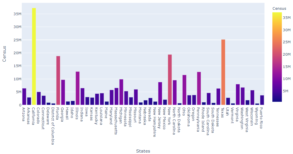
Now its time to plot the data
import plotly.express as px
data = px.data.gapminder()

fig = px.bar(df, x='States', y='Census',
             hover_data=['Census'], color='Census',
             labels={'pop':'population'}, height=400)
fig.show()
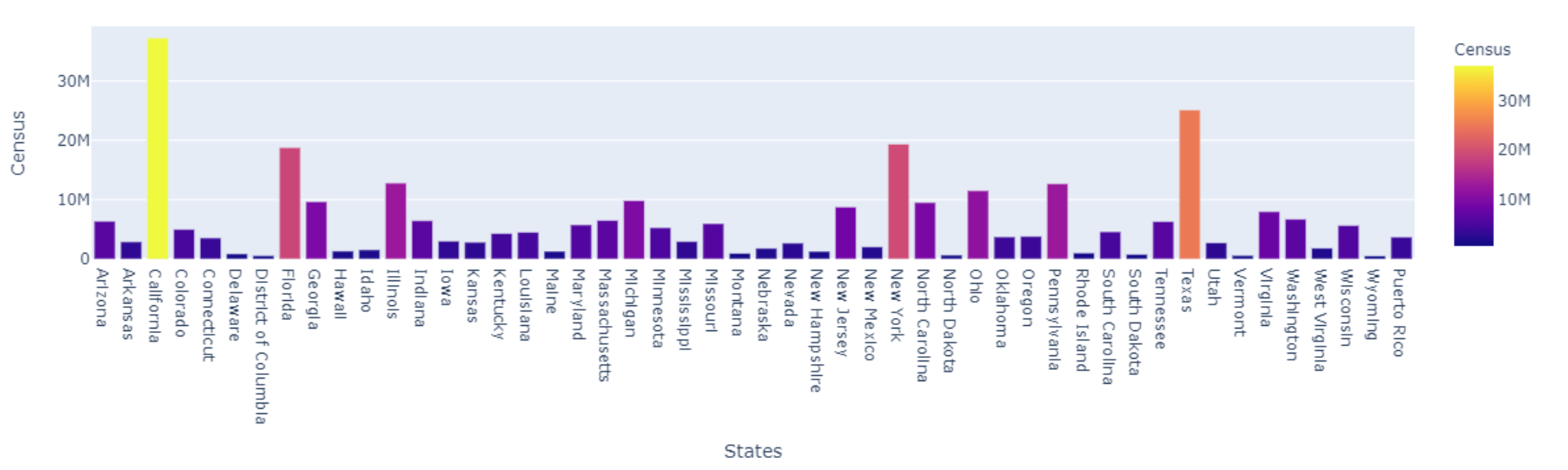
Tying it all together
import pandas as pd
import numpy as np

df = pd.read_excel('https://www2.census.gov/programs-surveys/popest/tables/2010-2019/state/totals/nst-est2019-01.xlsx')
new_header = df.iloc[2]
df = df[10:-5]
df.dropna(inplace = True)
df = df.replace('[^a-zA-Z0-9 ]', '', regex=True)
df.columns = new_header
df.rename(columns = {np.NaN : 'States'}, inplace= True)

import plotly.express as px
data = px.data.gapminder()

fig = px.bar(df, x='States', y='Census',
             hover_data=['Census'], color='Census',
             labels={'pop':'population'}, height=400)
fig.show()
As always, you can open an interactive version of this notebook at mybinder.org